Introduction
This is post four of a multi-part analysis of college basketball game outcomes. There are probably going to be things I mention in this post that I talked about in prior posts, so here are the links if you need to catch up.
This post specifically talks about a non-hierarchical clustering method, kmeans clustering. The concept behind kmeans clustering is relatively simple, and can generally be broken down into a few steps.
- Partition your data into K random, initial clusters. Each of the K clusters will have a centroid. Then centroid is the p dimensional mean vector of that cluster, where p is the number of variables that are in the data set.
- For each point in the data set, calculate the distance to each of the K centroids. Typically, this is the Euclidean distance, but other distances are applicable. Assign each point to cluster with the nearest centroid.
- Recalculate each of the K centroids.
- Repeat steps 2 and 3 until no points are assigned to a different cluster
This is an oversimplification of the algorithm applied here. I use the Hartigan-Wong algorithm in this demonstration, more details on the algorithm can be found here.
Preparing the Data
The data in this analysis is the output of post 3. I pulled that in using the connection from the r code chunk and SQL code chunk below.
base_dir <- '~/ncaa_data'
db_connection <- dbConnect(
      drv = RSQLite::SQLite(),
      dbname = file.path(base_dir, 'database.sqlite')
)
SELECT
*
FROM
clean_gamesFor clustering, I want my data to be clean, complete, and numeric. When I think about it, it doesn’t make sense to have non-numeric values in this algorithm. Say for example, we have a categorical variable, sex. How does one quantify the Euclidean distance between male and female?
For this reason, I want to remove rows with nulls, and any other data quality issues. From my own research and reading, it is not necessary to scale your data before clustering. With that being said, I think it should be done in most scenarios. A paper by Mohamad and Usman on standardization is a good reference, and can be found here.
# Remember to disconnect from db...
dbDisconnect(db_connection)


ds <- ds %>%
  filter(complete.cases(.)) %>%
  filter(
    is.finite(games.astto_season_avg_t1),
    is.finite(games.astto_season_avg_t2)
  )
For clustering, I want my data to be clean, complete, and numeric. When I think about it, it doesn’t make sense to have non-numeric values in this algorithm. Say for example, we have a categorical variable, sex. How does one quantify the Euclidean distance between male and female?
For this reason, I want to remove rows with nulls, and any other data quality issues. From my own research and reading, it is not necessary to scale your data before clustering. With that being said, I think it should be done in most scenarios. A paper by Mohamad and Usman on standardization is a good reference, and can be found here.
# Remember to disconnect from db...
dbDisconnect(db_connection)


ds <- ds %>%
  filter(complete.cases(.)) %>%
  filter(
    is.finite(games.astto_season_avg_t1),
    is.finite(games.astto_season_avg_t2)
  )

# Numeric only,
ds_fit <- ds%>%
  select(
    -id,
    -team1,
    -team2,
    -game_date,
    -season_t1,
    -games.outcome_t1,
    -games.tourney_t1,
    -games.home_t1,
    -games.away_t1,
    -games.neutral_t1,
    -season_t2
  ) %>%
  mutate_all(~scale(.)) %>%
  mutate_all(~round(., 4))
Deciding how many clusters
Long story short, I haven’t come across a golden rule for deciding this number.
The idea behind clustering is to from intelligent and meaningful clusters within the data. To do this, we want to maximize the variability between our clusters, but minimize the variability within each of the clusters. We define the sum of squares ratio as
\[SS_{ratio} = \frac{SS_{between}}{SS_{total}}\]
As we increase K, \(SS_{ratio}\) will approach 1. So we have to pick the amount of clusters that gives us the most bang for our buck. This can be done using the elbow method. The elbow method starts by calculating \(SS_{ratio}\) for an increasing number of clusters, K. I will start by initializing a vector to store the results.
ss_ratio <- rep(NA, 14)Now I want to fit a kmeans object with K clusters for all \(K \in (2 ... 15)\). For each K, I want to store the \(SS_{ratio}\) in the ss_ratio object I just initialized.
for(k in 2:(length(ss_ratio) + 1)) {
  fiti <- kmeans(
    x = ds_fit,
    centers = k,
    algorithm = 'Hartigan-Wong',
    iter.max = 100,
    nstart = 15
  )
  ss_ratio[k] <- fiti$betweenss / fiti$totss
}
Now that we have this vector containing the \(SS_{ratio}\) for each K, lets plot it using ggplot. I really like dark themed plots, and I found one I really liked on gitub.
# url to gist
url <- 'https://gist.githubusercontent.com/jslefche/eff85ef06b4705e6efbc/raw/736d3dc9fe71863ea62964d9132fded5e3144ad7/theme_black.R'

# download the code from the url and run it
eval(
  url %>%
    RCurl::getURL() %>%
    parse(text = .)
)


tibble(
  centroids = seq(2, length(ss_ratio) + 1),
  ss_ratio = ss_ratio
) %>%
  filter(centroids > 2) %>%
  ggplot(aes(x = centroids, y = ss_ratio)) +
    geom_line(color = '#08F7FE', size = 1.5, alpha = 0.75) +
    geom_point(color = '#08F7FE', size = 2.5, alpha = 0.75) +
    scale_x_continuous(breaks = seq(2, length(ss_ratio) + 1)) +
    labs(
      x = 'Number of Centroids',
      y = 'Between Sum of Squares Ratio',
      title = 'Between Sum of Squares Ratio',
      subtitle = 'For an increasing number of centroids'
    ) +
    theme_black()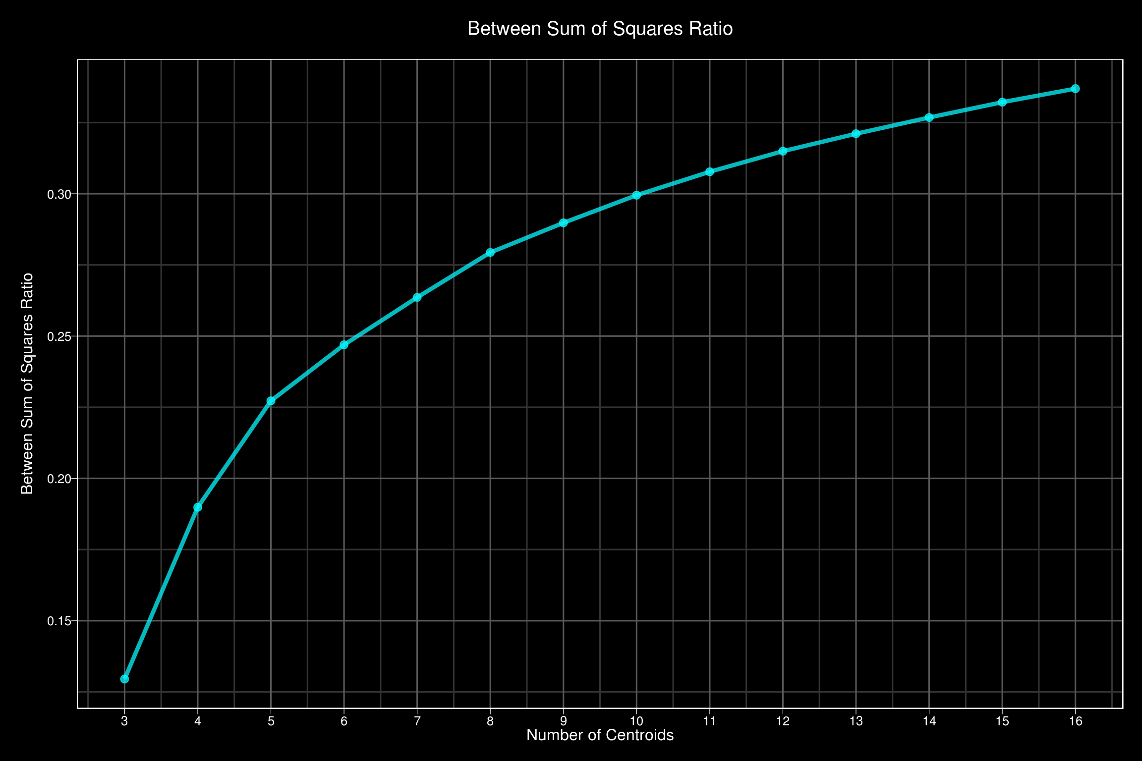
In this example, there isn’t a strong elbow, but we are essentially looking for a sharp bend in the plot. This one is more gradual. Five clusters looks good to me.
Now that we have chosen \(K = 5\), we will fit our kmeans object for 5 clusters.
set.seed(12)
fit <- kmeans(
    x = ds_fit,
    centers = 5,
    algorithm = 'Hartigan-Wong',
    iter.max = 200,
    nstart = 25
)
Now the fit object has a few different elements to it, but I am most interested in ‘cluster’. This is a vector of each data points cluster assignment. I want to take this, and plop it onto the data set that we started with, so that we can visualize the results.
ds$cluster <- fit$cluster

ds %>%
  mutate(cluster = as.factor(cluster)) %>%
  select(
    cluster,
    contains('t1'),
    -season_t1,
    -games.tourney_t1,
    -games.home_t1,
    -games.away_t1,
    -games.neutral_t1
  ) %>%
  ggpairs(
    aes(color = cluster),
    columns = 3:8,
    progress = FALSE,
    lower = list(continuous = wrap('smooth', alpha = 0.5)),
    diag = list(continuous = wrap('barDiag', alpha = 0.9, bins = 20))
  ) +
  labs(
    title = 'Pairs Plots for Team 1 Stats',
    subtitle = '**colored by resulting cluster**'
  ) +
  theme_black()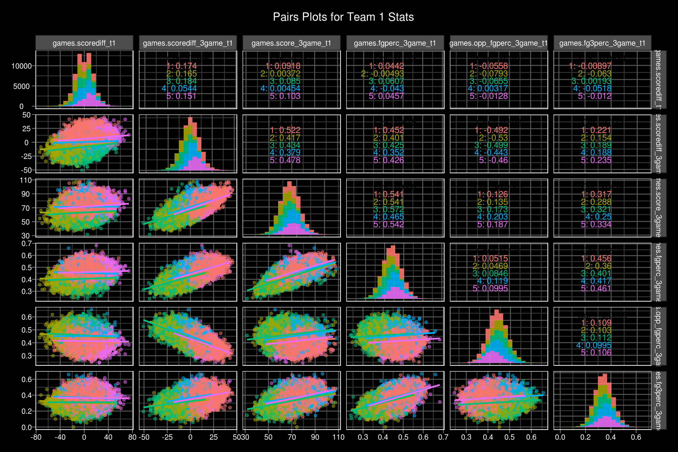
ds %>%
  mutate(cluster = as.factor(cluster)) %>%
  select(
    cluster,
    contains('t2'),
    -season_t1
  ) %>%
  ggpairs(
    aes(color = cluster),
    columns = 3:8,
    progress = FALSE,
    lower = list(continuous = wrap('smooth', alpha = 0.5)),
    diag = list(continuous = wrap('barDiag', alpha = 0.9, bins = 20))
  ) +
  labs(
    title = 'Pairs Plots for Team 2 Stats',
    subtitle = '**colored by resulting cluster**'
  ) +
  theme_black()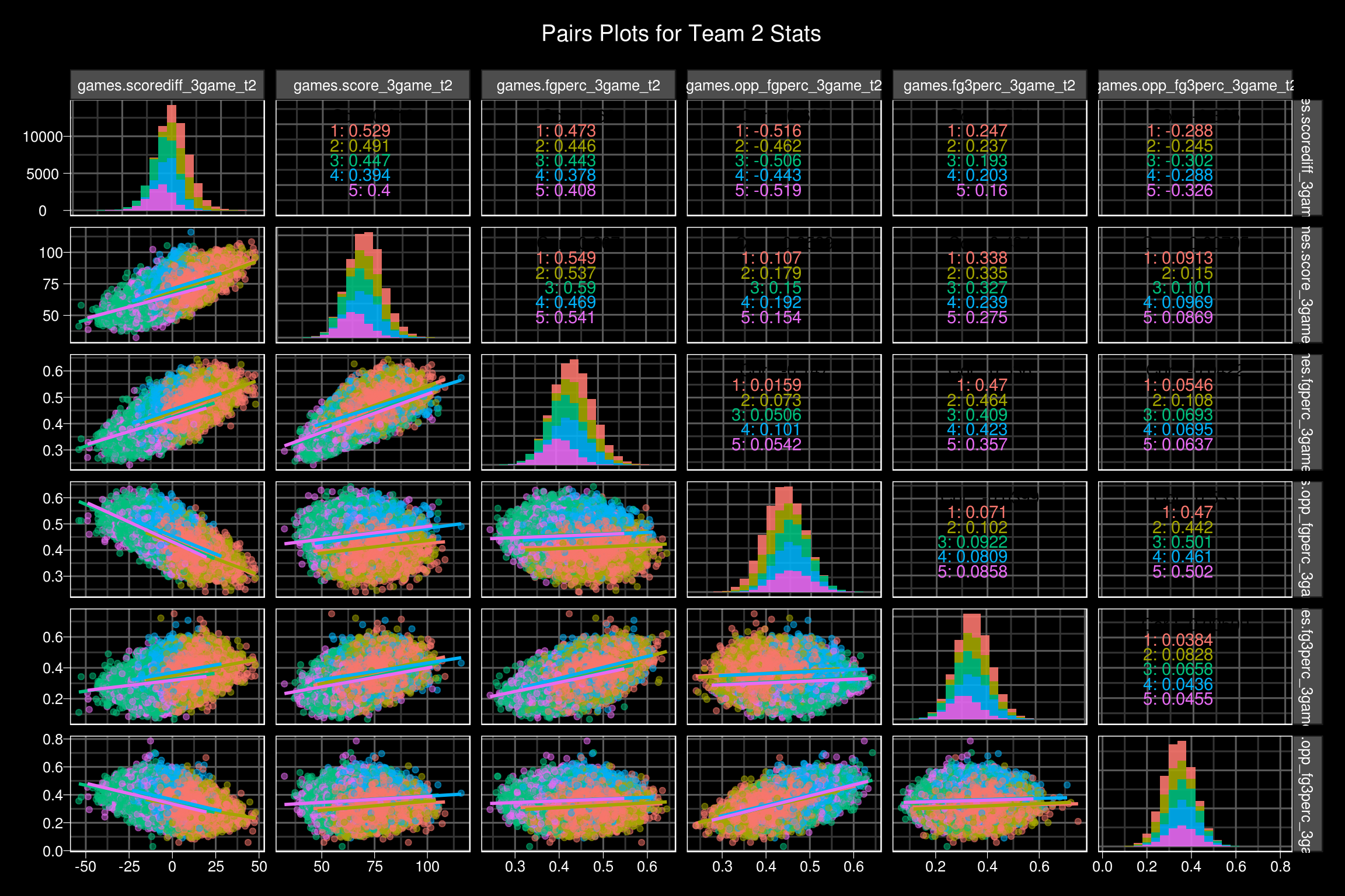
I love the GGally::ggpairs function. It really helps to see relationships between multiple variables at once.
I want to see the characteristics of the resulting clusters. Specifically, which clusters make it easy to pick a winner?
ds %>%
  mutate(
    outcome = case_when(
      games.scorediff_t1 > 0 ~ 'T1',
      TRUE ~ 'T2'
    )
  ) %>%
  group_by(cluster) %>%
  summarize(
    count = n(),
    avg_score_diff = mean(games.scorediff_t1),
    T1_wins = sum(outcome == 'T1'),
    T2_wins = sum(outcome == 'T2')
  ) %>%
  mutate(
    T1_win_rate = round(100 * T1_wins / count, 1),
    T2_win_rate = round(100 * T2_wins / count, 1)
  ) %>%
  select(cluster, T1_win_rate, T2_win_rate) %>%
  rename(
    Cluster = cluster,
    `Team 1 Win Percentage` = T1_win_rate,
    `Team 2 Win Percentage` = T2_win_rate
  ) %>%
   mutate(
    Cluster = cell_spec(
      Cluster,
      color = 'white',
      bold = TRUE,
      background = spec_color(
        Cluster,
        option = 'D',
        direction = -1
      )
    )
  ) %>%
  mutate_if(is.numeric, function(x) {
    cell_spec(
      x,
      bold = T,
      color = case_when(
        x >= 60 ~ 'green',
        x <= 40 ~ 'red',
        TRUE ~ 'grey'
      ),
      font_size = ifelse(x >= 60 | x <= 40, 16, 12)
    )
  }) %>%
  kable('html', escape = FALSE) %>%
  kable_styling(
    bootstrap_options = c("striped", "hover")
  ) %>%
add_header_above(c('Cluster Winning Percentages' = 3))| Cluster | Team 1 Win Percentage | Team 2 Win Percentage |
|---|---|---|
| 1 | 51.3 | 48.7 |
| 2 | 21.3 | 78.7 |
| 3 | 49.8 | 50.2 |
| 4 | 50.1 | 49.9 |
| 5 | 78.2 | 21.8 |
Here we can see cluster 2 and cluster 5 both have high win percentages for one of the teams. Lets see the some more detailed characteristics between the teams in each cluster.
table <- tibble()

for(i in unique(ds$cluster)){
  temp_t1_stats <- ds %>%
    filter(cluster == i) %>%
    select(
      contains('t1'),
      -season_t1,
      -games.outcome_t1,
      -games.tourney_t1,
      -games.home_t1,
      -games.neutral_t1,
      -games.away_t1,
      -games.scorediff_t1
    ) %>%
    summarize_all(~mean(.))

  temp_t2_stats <- ds %>%
    filter(cluster == i) %>%
    select(
      contains('t2'),
      -season_t2
    ) %>%
    summarize_all(~mean(.))


  colnames(temp_t1_stats) <- colnames(temp_t1_stats) %>%
    str_remove('_t1') %>%
    str_replace_all('_', ' ') %>%
    str_replace_all('\\.', ' ')

  colnames(temp_t2_stats) <- colnames(temp_t2_stats) %>%
    str_remove('_t2') %>%
    str_replace_all('_', ' ') %>%
    str_replace_all('\\.', ' ')

  table <- bind_rows(
    table,
    bind_rows(
      temp_t1_stats,
      temp_t2_stats,
      temp_t1_stats - temp_t2_stats
    ) %>%
    mutate_at(vars(contains('perc')), funs(. * 100)) %>%
    mutate_all(~round(., 2)) %>%
    mutate_at(vars(contains('perc')), funs(paste0(., '%'))) %>%
    mutate(Team = c('Team 1', 'Team 2', 'Difference'), Cluster = i) %>%
    select(Cluster, Team, everything())
  )
}

table %>%
  arrange(Cluster) %>%
  mutate(
    Cluster = cell_spec(
      Cluster,
      color = 'white',
      bold = TRUE,
      background = spec_color(
        Cluster,
        option = 'D',
        direction = -1
      )
    )
  ) %>%
  kable('html', escape = FALSE) %>%
  kable_styling(
    bootstrap_options = c("striped", "hover")
  ) %>%
  row_spec(
    seq(3, 15, 3),
    bold = TRUE,
    background = '#787878',
    color = 'white'
  ) %>%
  add_header_above(c('Cluster Team Stats Comparisons' = 22)) %>%
scroll_box(width = "100%", height = '400px') | Cluster | Team | games scorediff 3game | games score 3game | games fgperc 3game | games opp fgperc 3game | games fg3perc 3game | games opp fg3perc 3game | games ftperc 3game | games ordiff 3game | games drdiff 3game | games astto 3game | games scorediff season avg | games score season avg | games fgperc season avg | games opp fgperc season avg | games fg3perc season avg | games opp fg3perc season avg | games ftperc season avg | games ordiff season avg | games drdiff season avg | games astto season avg |
|---|---|---|---|---|---|---|---|---|---|---|---|---|---|---|---|---|---|---|---|---|---|
| 1 | Team 1 | 9.13 | 73.82 | 46.6% | 40.9% | 36.91% | 31.95% | 70.43% | 0.18 | 3.31 | 1.29 | 9.72 | 9.72 | 46.41% | 40.82% | 36.14% | 32.22% | 69.55% | 0.56 | 3.21 | 1.25 |
| 1 | Team 2 | 8.50 | 73.42 | 46.42% | 41.11% | 36.71% | 32.17% | 70.29% | 0.23 | 3.12 | 1.27 | 9.33 | 9.33 | 46.27% | 40.91% | 36.06% | 32.33% | 69.48% | 0.59 | 3.11 | 1.23 |
| 1 | Difference | 0.62 | 0.40 | 0.19% | -0.2% | 0.21% | -0.22% | 0.13% | -0.05 | 0.20 | 0.02 | 0.39 | 0.39 | 0.14% | -0.09% | 0.09% | -0.11% | 0.07% | -0.03 | 0.09 | 0.01 |
| 2 | Team 1 | -7.09 | 63.26 | 40.53% | 45.26% | 30.93% | 35.57% | 66.8% | 0.29 | -2.65 | 0.90 | -5.17 | -5.17 | 41.47% | 44.6% | 32.07% | 34.87% | 66.92% | 0.01 | -1.75 | 0.91 |
| 2 | Team 2 | 7.51 | 72.52 | 46.19% | 41% | 36.61% | 31.84% | 69.73% | -0.10 | 2.95 | 1.20 | 6.34 | 6.34 | 45.46% | 41.5% | 35.61% | 32.5% | 69.12% | 0.20 | 2.26 | 1.14 |
| 2 | Difference | -14.60 | -9.26 | -5.66% | 4.26% | -5.68% | 3.73% | -2.93% | 0.39 | -5.60 | -0.30 | -11.51 | -11.51 | -3.99% | 3.1% | -3.54% | 2.38% | -2.2% | -0.20 | -4.01 | -0.24 |
| 3 | Team 1 | -8.33 | 63.15 | 40.43% | 45.78% | 31.06% | 35.94% | 66.3% | 0.01 | -3.04 | 0.85 | -8.64 | -8.64 | 40.6% | 45.7% | 31.65% | 35.53% | 66.31% | -0.32 | -2.91 | 0.84 |
| 3 | Team 2 | -7.79 | 63.63 | 40.75% | 45.69% | 31.45% | 35.88% | 66.55% | 0.01 | -2.80 | 0.86 | -8.27 | -8.27 | 40.72% | 45.59% | 31.8% | 35.44% | 66.39% | -0.30 | -2.77 | 0.84 |
| 3 | Difference | -0.54 | -0.48 | -0.32% | 0.1% | -0.39% | 0.06% | -0.25% | 0.00 | -0.25 | -0.01 | -0.37 | -0.37 | -0.12% | 0.11% | -0.15% | 0.09% | -0.08% | -0.02 | -0.14 | 0.00 |
| 4 | Team 1 | 0.48 | 71.41 | 45.33% | 45.14% | 36.89% | 36.24% | 70.89% | -0.35 | -0.06 | 1.14 | -0.61 | -0.61 | 44.21% | 44.7% | 35.41% | 35.3% | 69.64% | -0.30 | -0.40 | 1.06 |
| 4 | Team 2 | 0.33 | 71.41 | 45.3% | 45.22% | 36.98% | 36.46% | 70.93% | -0.34 | -0.12 | 1.14 | -0.58 | -0.58 | 44.23% | 44.68% | 35.46% | 35.36% | 69.61% | -0.32 | -0.42 | 1.06 |
| 4 | Difference | 0.15 | 0.00 | 0.03% | -0.08% | -0.09% | -0.22% | -0.04% | -0.01 | 0.07 | 0.01 | -0.03 | -0.03 | -0.02% | 0.02% | -0.05% | -0.06% | 0.02% | 0.03 | 0.02 | 0.00 |
| 5 | Team 1 | 6.96 | 72.14 | 46.05% | 41.22% | 36.4% | 31.93% | 69.87% | -0.05 | 2.87 | 1.18 | 5.65 | 5.65 | 45.31% | 41.72% | 35.49% | 32.65% | 69.13% | 0.21 | 2.12 | 1.13 |
| 5 | Team 2 | -7.48 | 63.09 | 40.48% | 45.41% | 30.89% | 35.72% | 66.72% | 0.24 | -2.76 | 0.88 | -5.77 | -5.77 | 41.31% | 44.78% | 32.02% | 34.96% | 66.84% | -0.05 | -1.93 | 0.89 |
| 5 | Difference | 14.44 | 9.05 | 5.57% | -4.19% | 5.51% | -3.79% | 3.15% | -0.29 | 5.63 | 0.30 | 11.42 | 11.42 | 4% | -3.06% | 3.47% | -2.31% | 2.29% | 0.26 | 4.05 | 0.24 |
As expected, cluster two and cluster 5 show pretty drastic differences between the team 1 and team 2 statistics. In both clusters, there is about a 14 point difference in the teams 3 game rolling average score differential. Cluster two favors team two across the board, whereas cluster 5 favors team 1 in a similar fashion. Clusters 1, 3, and 4 are much more balanced. Cluster 1 and cluster 4 seem like high power offenses going at it, where as cluster 3 seems to be more geared towards lower powered offenses, due to the rolling 3 game scoring averages and shooting percentages.
Wrap Up
A cluster analysis is a good way to begin understanding your data. If you would’ve asked me before this analysis, I probably would’ve told you that this data could naturally be clustered into 3 groups: Team 1 wins easy, Team 2 wins easy, or it was a close game. That is essentially what happened. Clusters 2 and 5 represent those easy wins. The team with the better incoming statistics was more likely to win the game. Clusters 1, 3, and 4, were different flavors of close games.