NCAA Basketball Analysis Part 6 - Regression Tasks with Keras

Introduction

This is post 6 of a multi-part analysis of college basketball game outcomes. There are probably going to be things I mention in this post that I talked about in prior posts, so here are the links if you need to catch up.

• Post 1: Data Prep
• Post 2: Understanding the Dataset
• Post 3: Data Preprocessing
• Post 4: A Cluster Analysis
• Post 5: A Simple Neural Network With Keras

Last post showed how to use Keras for a classification task by classifying wins and losses. In this post, we are going to attack a regression task by modeling the point differential. I won’t explain in as great of detail in this post, for that, refer to post 5.

Building a Neural Network for Regression

base_dir <- '~/ncaa_data'
db_connection <- dbConnect(
  drv = RSQLite::SQLite(), 
  dbname = file.path(base_dir, 'database.sqlite')
)

SELECT 
*
FROM 
training

SELECT 
*
FROM 
testing

dbDisconnect(db_connection)

x_train <- training %>% 
  select(-games.outcome_t1, -games.scorediff_t1) %>% 
  as.matrix()

y_train <- training %>% 
  select(games.scorediff_t1) %>% 
  magrittr::extract2(1)

x_test <- testing %>% 
  select(-games.outcome_t1, -games.scorediff_t1) %>% 
  as.matrix()

y_test <- testing %>% 
  select(games.scorediff_t1) %>% 
  magrittr::extract2(1)

We are starting with the same training and testing data that we used in post 5. Now the modeling piece of this is going to be very similar to when classifying outcomes. The main difference comes with the activation function of the output layer. Recall, when working with a binary classification task, our activation function for the output layer was the sigmoid function. This returned a value between 0 and 1, which represented the probability of team 1 being the winning team. In this post, I would like to model the point differential. This outcome can technically be any integer value, so the sigmoid function will not work. To accomplish this, we will use a linear activation function.

model_build <- function(hyper_grid_i, input_shape) {
  model <- keras_model_sequential()
  
  model %>% 
    layer_dense(
      units = hyper_grid_i$units,
      activation = 'relu',
      kernel_initializer = 'normal',
      kernel_regularizer = regularizer_l2(l = hyper_grid_i$l2),
      input_shape = input_shape
    ) %>% 
    layer_dropout(hyper_grid_i$drop_rate) %>% 
    layer_dense(
      units = hyper_grid_i$units,
      activation = 'relu',
      kernel_initializer = 'normal',
      kernel_regularizer = regularizer_l2(l = hyper_grid_i$l2),
    ) %>% 
    layer_dropout(hyper_grid_i$drop_rate) %>% 
    layer_dense(
      units = hyper_grid_i$units,
      activation = 'relu',
      kernel_initializer = 'normal',
      kernel_regularizer = regularizer_l2(l = hyper_grid_i$l2),
    ) %>% 
    layer_dropout(hyper_grid_i$drop_rate) %>% 
    layer_dense(
      units = 1,
      # Notice the change in the activation function
      activation = 'linear',
      kernel_initializer = 'normal',
      kernel_regularizer = NULL
    ) %>% 
    compile(
      optimizer = optimizer_adam(lr = hyper_grid_i$adam_lr),
      loss = 'mean_squared_error',
      metric = 'mean_absolute_error'
    )
  
  return(model)
  
}

I’m going to use the same functions as the last post that helped me with my hypergrid search, with a slight modification to the fitNeval function. I first want to return the mean absolute error. I also want to use the continuous prediction to classify who is predicted to win/lose the game, and get the classification accuracy as well.

fitNeval <- function(model, x_train, y_train, x_test, y_test, epochs_i) {
  fit(
    object = model,
    x = x_train,
    y = y_train,
    batch_size = 100,
    epochs = epochs_i,
    verbose = 0
  )
  
  estimate <- model %>% predict(x_test)
  
  # Added functionality to calculate mae
  mae <- tibble(y_test, estimate) %>% 
    # Avoiding predictions of 0 
    mutate(
      estimate = case_when(
        estimate > 0 & estimate < 1 ~ 1,
        estimate > -1 & estimate < 0 ~ -1,
        TRUE ~ round(estimate, 0)
      )
    ) %>% 
    yardstick::mae(truth = y_test, estimate = estimate) %>% 
    magrittr::extract2(3)
  
  accuracy <- tibble(
    truth = if_else(y_test > 0, 1, 0),
    estimate = if_else(estimate > 0, 1, 0)
  ) %>% 
    yardstick::accuracy(truth = as.factor(truth), estimate = as.factor(estimate)) %>% 
    magrittr::extract2(3)
  
  results <- list(accuracy = accuracy, mae = mae)
  
  
  return(results)
}

Now that our functions are set up, and our hyper grid defined, we can loop through the hyper_grid.

results <- tibble(i = integer(), accuracy = double(), mae = double())  

for (i in 1:nrow(hyper_grid)) {
  
  tmp_model <- model_build(hyper_grid[i,], ncol(x_train))
  
  tmp_metrics <- fitNeval(
    tmp_model, 
    x_train = x_train, 
    x_test = x_test, 
    y_train = y_train, 
    y_test = y_test,
    epochs_i = hyper_grid$epochs[i]
  )
  
  
  results <- bind_rows(
    results, 
    tibble(
      i = i, 
      accuracy = tmp_metrics$accuracy, 
      mae = tmp_metrics$mae
    )
  )
}

Now that we have searched over a grid of hyper parameters, we can select which set minimizes the mae.

# Extracting to hyper-parameters
top_params <- results %>% arrange(mae) %>% slice(1)

# Build model with optimal hyper-parameters
model <- model_build(top_params, input_shape = ncol(x_train))

# Fit the model 
history <- fit(
  object = model,
  x = x_train,
  y = y_train,
  batch_size = 100,
  epochs = 25,
  verbose = 0
)

T1_scorediff_estimate <- predict(object = model, x = x_test)
T1_scorediff_estimate <- case_when(
  T1_scorediff_estimate > 0 & T1_scorediff_estimate < 1 ~ 1,
  T1_scorediff_estimate > -1 & T1_scorediff_estimate < 0 ~ -1,
  TRUE ~ round(T1_scorediff_estimate, 0)
)

T1_win_class_estimate <- if_else(T1_scorediff_estimate > 0, 1, 0)
y_test_class <- if_else(y_test > 0, 1, 0)

mae <- bind_cols(
  truth = y_test,
  estimate = T1_scorediff_estimate
) %>% yardstick::mae(truth = truth, estimate = estimate)

accuracy <- bind_cols(
  truth = as.factor(y_test_class),
  estimate = as.factor(T1_win_class_estimate)
) %>% yardstick::accuracy(truth = truth, estimate = estimate)

bind_rows(mae, accuracy) %>% 
  kable('html') %>% 
  kable_styling(
    bootstrap_options = c("striped", "hover")
  )

The accuracy is very similar to the best accuracy obtained when specifically trying to classify the outcome. The nice part about this model is that we can also estimate the point differential, which has a mean absolute error of about 9 points.

bind_cols(
  truth = y_test,
  estimate = T1_scorediff_estimate
) %>% 
  mutate(
    error = y_test - T1_scorediff_estimate
  ) %>% 
  ggplot(aes(x = error, )) +
  geom_histogram(
    aes(y=..count../sum(..count..)), 
    binwidth = 5,
    color = 'white'
  ) + 
  scale_x_continuous(
    breaks = seq(-40, 40, 5)
  ) +
  labs(
    x = 'Estimated Point Differential',
    y = 'Proportion of games',
    title = 'Residual Distribution'
  ) +
  ggthemes::theme_economist()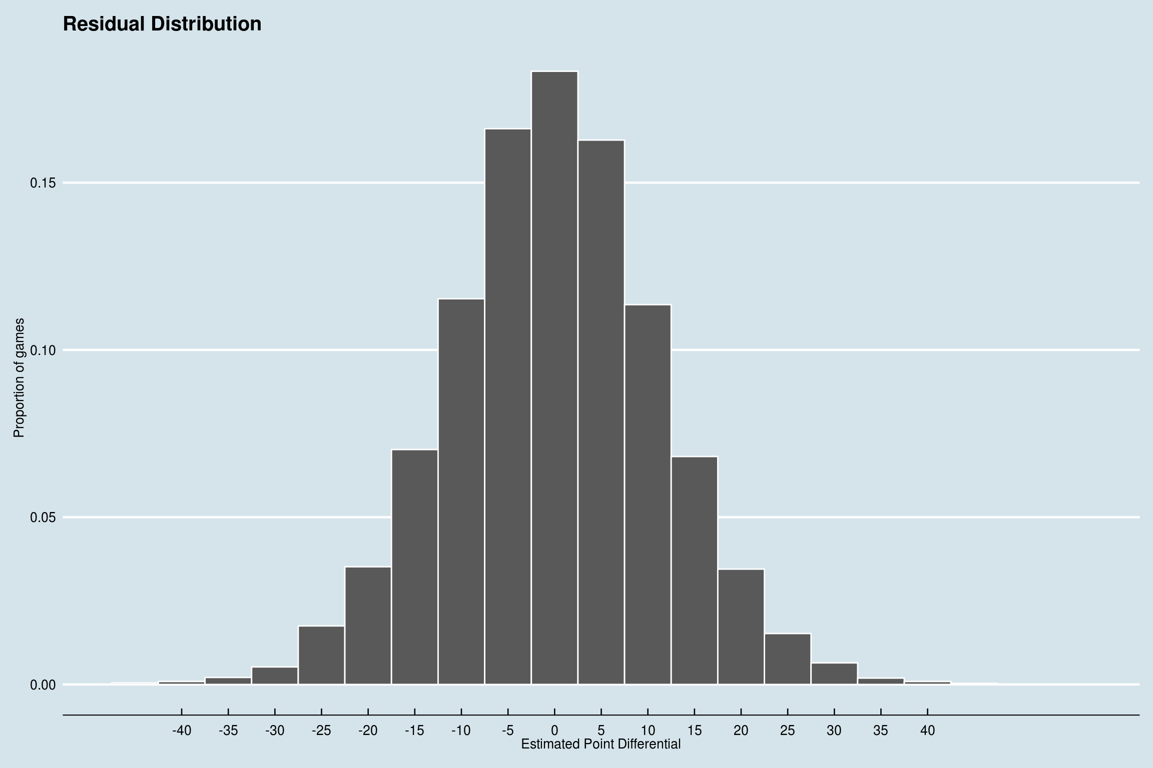

Here we can see how the residuals are distributed. There are a handfull of games that are wildly off, but overall, the predictions aren’t bad. Out of 15836, 66% of predictions were within 10 points, and only 7 were off by more than 20.

Conclusion

So I know this post was a lot lighter on descriptions and explanations, but post 5 covered what I wanted to talk about from that perspective, so take a look there if you want some more info.

Overall, I am not all that surprised that these models didn’t do better. With the data that we had, and the feature engineering that we have done so far, I think low to mid 70s in terms of prediction accuracy is pretty good. There is so much that goes into who is going to win a basketball game. And upsets happen all the time.

Next post will be pretty similar, I am going to look at the same two tasks I talked about in the last two posts, except I am going to use xgboost instead. See ya next time!