Introduction
This is post four of a multi-part analysis of college basketball game outcomes. There are probably going to be things I mention in this post that I talked about in prior posts, so here are the links if you need to catch up.
- Post 1: Data Prep
- Post 2: Understanding the Dataset
- Post 3: Data Preprocessing
- Post 4: A Cluster Analysis
One of the end products of this series of posts is going to be a handful of models that predict the outcome of a given game. I am going to start by attempting to classify wins and losses, and will progress to estimating the point differential. This post is geared specifically towards building a multi-layer perceptron for classification using keras. Neural networks require a lot of detail and can be dificult to learn. I am not going to go into crazy detail for some of the steps, but I will provide links to a few of the places that I found inspiration as well as great explanations.
Query and Preprocessing the Data
The data pull is the same as in my other posts. If you don’t have the data set, refer to the links to the previous posts above to see how I did it.
base_dir <- '~/ncaa_data'
db_connection <- dbConnect(
      drv = RSQLite::SQLite(),
      dbname = file.path(base_dir, 'database.sqlite')
)
SELECT
*
FROM
clean_gamesAs of right now, we have a handfull of records that are incomplete, and two records that showed an infinite assist to turnover ratio. While obviously that is not possible, it only accounts for 6 records out of ~ 60 thousand records, so I just filtered them out. I may go back and try to troubleshoot it later…
ds <- ds %>%
  filter(complete.cases(.)) %>%
  filter(
    is.finite(games.astto_season_avg_t1),
    is.finite(games.astto_season_avg_t2)
  ) %>%
  mutate_at(
    .vars = vars(
      id,
      team1,
      team2,
      game_date,
      season_t1,
      games.outcome_t1,
      games.tourney_t1,
      games.home_t1,
      games.away_t1,
      games.neutral_t1
    ),
    .funs = ~as.factor(.)
  ) %>%
  select(
    -id,
    -games.neutral_t1,
    -game_date,
    -games.tourney_t1,
    -team1,
    -team2,
    -season_t2
  )

ds %>%
  head(n = 5) %>%
  kable('html') %>%
  kable_styling(
    bootstrap_options = c("striped", "hover")
  ) %>%
scroll_box(width = "100%")| season_t1 | games.outcome_t1 | games.home_t1 | games.away_t1 | games.scorediff_t1 | games.scorediff_3game_t1 | games.score_3game_t1 | games.fgperc_3game_t1 | games.opp_fgperc_3game_t1 | games.fg3perc_3game_t1 | games.opp_fg3perc_3game_t1 | games.ftperc_3game_t1 | games.ordiff_3game_t1 | games.drdiff_3game_t1 | games.astto_3game_t1 | games.scorediff_season_avg_t1 | games.score_season_avg_t1 | games.fgperc_season_avg_t1 | games.opp_fgperc_season_avg_t1 | games.fg3perc_season_avg_t1 | games.opp_fg3perc_season_avg_t1 | games.ftperc_season_avg_t1 | games.ordiff_season_avg_t1 | games.drdiff_season_avg_t1 | games.astto_season_avg_t1 | games.scorediff_3game_t2 | games.score_3game_t2 | games.fgperc_3game_t2 | games.opp_fgperc_3game_t2 | games.fg3perc_3game_t2 | games.opp_fg3perc_3game_t2 | games.ftperc_3game_t2 | games.ordiff_3game_t2 | games.drdiff_3game_t2 | games.astto_3game_t2 | games.scorediff_season_avg_t2 | games.score_season_avg_t2 | games.fgperc_season_avg_t2 | games.opp_fgperc_season_avg_t2 | games.fg3perc_season_avg_t2 | games.opp_fg3perc_season_avg_t2 | games.ftperc_season_avg_t2 | games.ordiff_season_avg_t2 | games.drdiff_season_avg_t2 | games.astto_season_avg_t2 |
|---|---|---|---|---|---|---|---|---|---|---|---|---|---|---|---|---|---|---|---|---|---|---|---|---|---|---|---|---|---|---|---|---|---|---|---|---|---|---|---|---|---|---|---|---|
| 2003 | 1 | 0 | 0 | 25 | 34.33333 | 79.33333 | 0.4897973 | 0.2450065 | 0.4306418 | 0.2555556 | 0.6882333 | -8.000000 | 11.3333333 | 1.4471844 | 34.33333 | 34.33333 | 0.4897973 | 0.2450065 | 0.4306418 | 0.2555556 | 0.6882333 | -8.000000 | 11.333333 | 1.4471844 | -8.666667 | 65.66667 | 0.4687214 | 0.4975097 | 0.3115218 | 0.3751994 | 0.6616162 | 1.666667 | 1.666667 | 0.8249084 | -8.666667 | -8.666667 | 0.4687214 | 0.4975097 | 0.3115218 | 0.3751994 | 0.6616162 | 1.666667 | 1.666667 | 0.8249084 |
| 2003 | 1 | 1 | 0 | 8 | -17.33333 | 57.66667 | 0.4125122 | 0.4885150 | 0.1690717 | 0.4459064 | 0.6388889 | 3.000000 | 0.3333333 | 0.6957418 | -12.75000 | -12.75000 | 0.4515410 | 0.4814656 | 0.2614191 | 0.4480662 | 0.6837121 | 0.500000 | 1.500000 | 0.8218063 | -30.000000 | 54.33333 | 0.3277788 | 0.5102682 | 0.2004177 | 0.4719298 | 0.5996757 | 8.000000 | -4.000000 | 0.6351236 | -30.000000 | -30.000000 | 0.3277788 | 0.5102682 | 0.2004177 | 0.4719298 | 0.5996757 | 8.000000 | -4.000000 | 0.6351236 |
| 2003 | 1 | 1 | 0 | 23 | 14.00000 | 72.33333 | 0.4514137 | 0.3671233 | 0.2698148 | 0.3170445 | 0.6483008 | 3.000000 | 4.6666667 | 1.4924242 | 14.00000 | 14.00000 | 0.4514137 | 0.3671233 | 0.2698148 | 0.3170445 | 0.6483008 | 3.000000 | 4.666667 | 1.4924242 | -11.000000 | 72.00000 | 0.4073730 | 0.5291736 | 0.3013291 | 0.4023810 | 0.7394444 | 2.000000 | -8.000000 | 1.3755991 | -11.000000 | -11.000000 | 0.4073730 | 0.5291736 | 0.3013291 | 0.4023810 | 0.7394444 | 2.000000 | -8.000000 | 1.3755991 |
| 2003 | 1 | 0 | 0 | 10 | 24.33333 | 84.00000 | 0.4758964 | 0.3787582 | 0.3489975 | 0.3157823 | 0.5640152 | 3.333333 | 6.0000000 | 1.3452381 | 23.50000 | 23.50000 | 0.5027556 | 0.3810074 | 0.3386712 | 0.2868367 | 0.5896780 | 1.500000 | 6.000000 | 1.2589286 | 17.333333 | 80.66667 | 0.4950017 | 0.4160751 | 0.3666667 | 0.3185185 | 0.6287538 | 6.333333 | 7.000000 | 1.0214931 | 17.333333 | 17.333333 | 0.4950017 | 0.4160751 | 0.3666667 | 0.3185185 | 0.6287538 | 6.333333 | 7.000000 | 1.0214931 |
| 2003 | 1 | 0 | 0 | 2 | 10.33333 | 77.00000 | 0.4682905 | 0.4485086 | 0.4533333 | 0.2208333 | 0.6829590 | -1.333333 | -3.3333333 | 1.1216330 | 10.33333 | 10.33333 | 0.4682905 | 0.4485086 | 0.4533333 | 0.2208333 | 0.6829590 | -1.333333 | -3.333333 | 1.1216330 | 15.666667 | 77.33333 | 0.4735300 | 0.3948347 | 0.5004810 | 0.3746499 | 0.6685315 | 5.333333 | 6.000000 | 1.0661376 | 8.750000 | 8.750000 | 0.4304900 | 0.3995743 | 0.4042069 | 0.3920985 | 0.6535725 | 7.500000 | 3.500000 | 0.9871032 |
As you can see above, we now have our few categorical variables one hot encoded, and the rest of our numbers we calculated in the previous posts. Now for a deep learning model, I typically center and scale my data. At first glance, I was going to apply this process while looking at the dataset as a whole. But the more I thought about this, the less that apprach made sense to me. This is mostly speculation, I don’t have the hard facts to back it up, but I would be willing to bet money that the game has changed a bit in the 14 season span of games we are looking at. To account for this, I wanted to center and scale the data, within each season. To do this, I used a for loop, and the recipes package. Small sidebar, I love the recipes package. So far, I have only used a handful of the steps that you can apply, but there are so many preprocessing steps you can apply. Even better, it is all contained in a single object, so I can move that recipe around and bake it wherever I need!
# Extracting list of seasons
seasons <- ds %>%
  select(season_t1) %>%
  distinct() %>%
  magrittr::extract2(1)

# Initializing storage for preprocessed data
store <- tibble()

# Looping through each season in seasons
for (season in seasons) {

  # Extract season from ds
  tmp <- ds %>% filter(season_t1 == season)

  # Center and scale all numeric variables
  rec <- tmp %>%
    recipe() %>%
    step_center(all_numeric(), -games.scorediff_t1) %>%
    step_scale(all_numeric(), -games.scorediff_t1) %>%
    prep(.)

  # Append that to the store object
  store <- bind_rows(store, rec %>% bake(tmp))

  # Rinse and repeat until all seasons have been preprocessed
}
Now the store object is the same size as the ds object that we were previously looking at, except store is centered and scaled with depending on the season. Now I don’t want the season variable to be used for prediction, so I am going to drop that here. I also want my factors back to numerics. I do this here so I can assure the data looks correct before converting to a matrix. I also want to shuffle my data. The data set in its curent state is ordered by date. To avoid this, I use slice and sample.
# Remove season, and hacky way back to numerics from factors
store <- store %>%
  select(-season_t1) %>%
  mutate_if(is.factor, as.character) %>%
  mutate_if(is.character, as.numeric)

# Shuffling the data set
store <- slice(store, sample(1:n()))
Now that I have the data set preprocessed, I want to split to a testing and training set. Since I will be building another classification model, I wanted to store the training and testing set to ensure we are comparing apples to apples when comparing the models. I also want to ensure that I have a very similar proportion of team 1 wins in the training and testing data, which is taken care of with the strata parameter in the initial_split function
# Splitting with rsample
split <- initial_split(store, prop = 3/4, strata = 'games.outcome_t1')
training <- training(split)
testing <- testing(split)

# Writing these to the database
dbWriteTable(
      conn = db_connection,
      name = 'training',
      value = training,
      overwrite = TRUE
)
dbWriteTable(
      conn = db_connection,
      name = 'testing',
      value = testing,
      overwrite = TRUE
)

# Remember to disconnect from db...
dbDisconnect(db_connection)
Modeling
Okay, now we are ready to model this data. I am using keras in this script to create a simple, multi-layer perceptron. I have used a few different frameworks, using both R and Python, and I really like using keras in R. I really like the tidyverse style piping to create the network. I’m not going to get into the explanation of how neural networks work, but I will share some of my favorite resources down at the bottom. One thing I really like about keras is how easy it is to tweak the model architecture and hyperparameters. To begin, I will build a simple network, to demonstrate a few of the hyperparameters that I like to control. I want to start by getting our data set in a way that keras understands. Keras uses the ideas of tensors, and I am not going to get into the details here. For this example, we need to separate our dataset into our input tensor and a vector of targets. Our input tensor will be our predictor variables as columns, and observations as rows, and will need to be of type matrix. Our training dataframe contains our predictor variables, as well as two potential targets; games.outcome_t1 and games.scorediff_t1.
x_train <- training %>%
  select(-games.outcome_t1, -games.scorediff_t1) %>%
  as.matrix()

y_train <- training %>%
  select(games.outcome_t1) %>%
  magrittr::extract2(1)

x_test <- testing %>%
  select(-games.outcome_t1, -games.scorediff_t1) %>%
  as.matrix()

y_test <- testing %>%
  select(games.outcome_t1) %>%
  magrittr::extract2(1)
Now we start building by first initializing the model object.
# Initializing model object
model <- keras_model_sequential()
Building a NN in keras has a feels a bit different thatn a lot of the models I have built using more traditional machine learning type packages. Instead of feeding parameters into a function, we build the structure of the model by piping the model object into functions that add layers to the model. Here, we are going to build a densely-connected multilayer perceptron. To do this, we will add densely connected layers using the layer_dense function.
There are a few parameters that I like to use / tweak when building with the layer_dense function, and they are shown below.
- object - this is required, and it is the model object initialized above.
- units - this is required, and this is the number of hidden units in the layer.
- activation - this is the activation function for this layer, no activation if nothing provided.
- kernel_regularizer - this allows us to add L1, L2, or L1 and L2 regularization to the layer.
- input_shape - only required on the first layer, and is the dimensionality of an observation of your input data.
Object is obvious, this is the model object, which we will pipe into the function. Units is a hyper-parameter that takes some searching. I will test out 16 hidden units here. I won’t give over-simplified explanations of the activation functions or regularization, but I will share some of my favorite articles about them below. One of the toughest concepts for me to understand at first was the input shape, and how the shape changes from layer to layer. The first layer requires the input_shape as a parameter, whereas keras is smart enough to take the output shape of the previous layer for the remaining densely connected layers. In our example, the input shape is the number of columns in x_train. This is because a single row of the input matrix maps to a single element of the target vector, y_train. Below is an example of adding a layer to a model.
# pass model object into layer_dense to add a densely connected layer
model %>%
  layer_dense(
    # number of hidden units
    units = 16,
    # activation function
    activation = 'relu',
    # adding l2 regularization
    kernel_regularizer = regularizer_l2(l = 0.01),
    # providing the input shape
    input_shape = ncol(x_train),
  )

# Printing a summary of the model
summary(model)
- ___________________________________________________________________________
- Layer (type) Output Shape Param #
- ===========================================================================
- dense_1 (Dense) (None, 16) 688
- ===========================================================================
- Total params: 688
- Trainable params: 688
- Non-trainable params: 0
- ___________________________________________________________________________As you can see, there is 1 layer, with 688 parameters. Our input shape was 1 x 42. We told the layer to have 16 hidden units. For each of the 42 variables have a weight, or a parameter, for each of the 16 hidden units. This takes us to 672 parameters. The remaining 16 are bis terms, one for each hidden unit.
Now I want to add a dropout layer to the model. This will help us avoid overfitting the model. The only parameter I use for the dropout layer is the rate, and occationally the seed.
model %>% layer_dropout(rate = 0.1)

summary(model)
- ___________________________________________________________________________
- Layer (type) Output Shape Param #
- ===========================================================================
- dense_1 (Dense) (None, 16) 688
- ___________________________________________________________________________
- dropout_1 (Dropout) (None, 16) 0
- ===========================================================================
- Total params: 688
- Trainable params: 688
- Non-trainable params: 0
- ___________________________________________________________________________As you can see, adding a dropout layer doesn’t change the output shape of the model, and doesn’t have any trainable parameters.
Now for the output layer. In this use case, we have a single output, the outcome of the game. This tells us how many units we need to have in the output layer. We need 1 unit per outcome. We are also going to switch up our activation function. For binary classification, we are going to use the sigmoid function. This will return a value between 0 and 1, representing the probability of team 1 winning the game.
model %>%
  # adding a hidden layer
  layer_dense(
    units = 16,
    activation = 'relu',
    kernel_regularizer = regularizer_l2(l = 0.01)
  ) %>%
  layer_dropout(rate = 0.1) %>%
  # output layer
  layer_dense(
      # single output
      units = 1,
      # sigmoid activation for classification
      activation = 'sigmoid'
  )

summary(model)
- ___________________________________________________________________________
- Layer (type) Output Shape Param #
- ===========================================================================
- dense_1 (Dense) (None, 16) 688
- ___________________________________________________________________________
- dropout_1 (Dropout) (None, 16) 0
- ___________________________________________________________________________
- dense_2 (Dense) (None, 16) 272
- ___________________________________________________________________________
- dropout_2 (Dropout) (None, 16) 0
- ___________________________________________________________________________
- dense_3 (Dense) (None, 1) 17
- ===========================================================================
- Total params: 977
- Trainable params: 977
- Non-trainable params: 0
- ___________________________________________________________________________As you can see, dense_2 has 272 parameters. Recall, the output shape of dense_1 was 16, because of our 16 hidden units. These 16 outputs feed into the 16 units of dense_2. So 16 outputs * 16 hidden units + 16 bias parameters brings us to 272 trainable parameters in dense_2. The output layer then has 16 outputs from the previous layer, times 1 hidden unit, plus 1 bias term, for a total of 17 trainable parameters in the output layer, for a total of 977 trainable parameters in the network. And thats a very simple model architecture! Now it’s time to define the optimizer and the loss function, and compile the model.
There are a few decisions that have to be made when fitting the model object. One is the number of epochs to perform, and the other being the batch size. An epoch consists of one full pass of training data through the model. The batch size is how many observations are passed into the model, before the model recalculates its weights. There are a few methodologies for setting these values. I’ll put some good links below.
model %>%
  compile(
      # using adam optimizer
      optimizer = 'adam',
      # binary crossentropy for classification
      loss = 'binary_crossentropy',
      metric = 'accuracy'
  )
history <- fit(
object = model,
x = x_train,
y = y_train,
batch_size = 100,
epochs = 20,
verbose = 0
)Now that we trained a model object, we can visualize the accuracy and the loss by epoch. Keras can do this with the plot function, but I like using ggplot so I plotted it that way.
p1 <- tibble(
    accuracy = history$metrics$acc,
    loss = history$metrics$loss
) %>%
    rowid_to_column('Epoch') %>%
    ggplot(aes(x = Epoch, y = accuracy)) +
    geom_point(size = 2, alpha = 0.75, color = '#08F7FE') +
    geom_smooth(method = 'loess', se = FALSE, color = '#F5D300') +
    labs(
        x = 'Epoch',
        y = 'Accuracy',
        title = 'Training Metrics'
    ) +
    ggdark::dark_theme_minimal()

p2 <- tibble(
    accuracy = history$metrics$acc,
    loss = history$metrics$loss
) %>%
    rowid_to_column('Epoch') %>%
    ggplot(aes(x = Epoch, y = loss)) +
    geom_point(size = 2, alpha = 0.75, color = '#08F7FE') +
    geom_smooth(method = 'loess', se = FALSE, color = '#F5D300') +
    labs(
        x = 'Epoch',
        y = 'Loss'
    ) +
    ggdark::dark_theme_minimal()

cowplot::plot_grid(p1, p2, nrow = 2)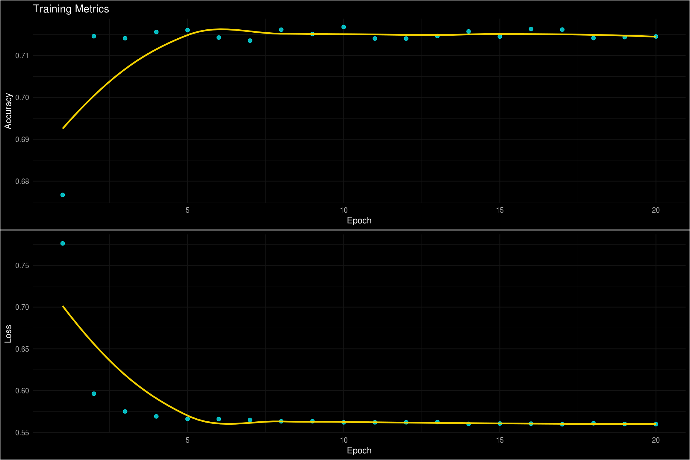
We can also evaluate the performance of the model using yardstick. Yardstick has a handful of functions for calculating a variety of model metrics. For classification, a few common metrics are classification, precision, and recall. Typically, precision and recall are better ways for me to evaluate the performance of a model. The reason being, there is typically a considerable cost of mis-classifying observations. This use case is a bit of a special case. Both outcomes really represent the same thing, so both scenarios should carry the same weight. For that reason, I am going to focus on accuracy for my metric that I am trying to maximize.
pred_probs <- predict_proba(object = model, x = x_test) %>%
    as.vector() %>%
    round(2)

estimate <- as.factor(ifelse(pred_probs > 0.5, 1, 0))

tibble(y_test, estimate) %>%
    yardstick::accuracy(truth = as.factor(y_test), estimate = estimate) %>%
    kable('html') %>%
    kable_styling(bootstrap_options = c("striped", "hover"))
Alright! So with now I want to get into the nitty-gritty on how I search for optimal models. One of the challenges we face is knowing what to set the hyper-parameters to. Most of the time, its a bit of trial and error. One way to do this is by doing a grid search. We will create a parameter space for all of the parameters that we are looking to optimize. In this example, we will search for a few of the hyper-parameters that we used to build the perceptron from above. Base R has a cool function, expand.grid, that makes this super easy. I am going to search for the optimal number of hidden units, the drop rate in the dropout layer, the learning rate of the adam optimizer, the L2 regularization factor, and the number of epochs.
hyper_grid <- expand.grid(
  units = c(16, 32, 64),
  drop_rate = c(0.1, 0.25, 0.5),
  adam_lr = c(0.0001, 0.00005),
  l2 = c(0.005, 0.01),
  epochs = c(25)
)

hyper_grid %>%
    kable('html') %>%
    kable_styling(bootstrap_options = c("striped", "hover")) %>%
    add_header_above(c("Hyper Grid Scenarios" = 5)) %>%
scroll_box(height = '400px') | units | drop_rate | adam_lr | l2 | epochs |
|---|---|---|---|---|
| 16 | 0.10 | 1e-04 | 0.005 | 25 |
| 32 | 0.10 | 1e-04 | 0.005 | 25 |
| 64 | 0.10 | 1e-04 | 0.005 | 25 |
| 16 | 0.25 | 1e-04 | 0.005 | 25 |
| 32 | 0.25 | 1e-04 | 0.005 | 25 |
| 64 | 0.25 | 1e-04 | 0.005 | 25 |
| 16 | 0.50 | 1e-04 | 0.005 | 25 |
| 32 | 0.50 | 1e-04 | 0.005 | 25 |
| 64 | 0.50 | 1e-04 | 0.005 | 25 |
| 16 | 0.10 | 5e-05 | 0.005 | 25 |
| 32 | 0.10 | 5e-05 | 0.005 | 25 |
| 64 | 0.10 | 5e-05 | 0.005 | 25 |
| 16 | 0.25 | 5e-05 | 0.005 | 25 |
| 32 | 0.25 | 5e-05 | 0.005 | 25 |
| 64 | 0.25 | 5e-05 | 0.005 | 25 |
| 16 | 0.50 | 5e-05 | 0.005 | 25 |
| 32 | 0.50 | 5e-05 | 0.005 | 25 |
| 64 | 0.50 | 5e-05 | 0.005 | 25 |
| 16 | 0.10 | 1e-04 | 0.010 | 25 |
| 32 | 0.10 | 1e-04 | 0.010 | 25 |
| 64 | 0.10 | 1e-04 | 0.010 | 25 |
| 16 | 0.25 | 1e-04 | 0.010 | 25 |
| 32 | 0.25 | 1e-04 | 0.010 | 25 |
| 64 | 0.25 | 1e-04 | 0.010 | 25 |
| 16 | 0.50 | 1e-04 | 0.010 | 25 |
| 32 | 0.50 | 1e-04 | 0.010 | 25 |
| 64 | 0.50 | 1e-04 | 0.010 | 25 |
| 16 | 0.10 | 5e-05 | 0.010 | 25 |
| 32 | 0.10 | 5e-05 | 0.010 | 25 |
| 64 | 0.10 | 5e-05 | 0.010 | 25 |
| 16 | 0.25 | 5e-05 | 0.010 | 25 |
| 32 | 0.25 | 5e-05 | 0.010 | 25 |
| 64 | 0.25 | 5e-05 | 0.010 | 25 |
| 16 | 0.50 | 5e-05 | 0.010 | 25 |
| 32 | 0.50 | 5e-05 | 0.010 | 25 |
| 64 | 0.50 | 5e-05 | 0.010 | 25 |
The hyper_grid dataframe has 36 rows, or scenarios to test. What I want to do now is define a loop to a model for each of scenarios defined above. I also want to test out a few more hidden layers. Before I do that, I want to define a few things. First, I am going to create a functions that defines a 3 layer model and a function that fits and evaluates the model. I also will create a tibble to store the results. First, lets look at what the model build function looks like. Putting this into a function is not necessary, but I prefer it because it makes the loop code a lot cleaner and easier to understand.
model_build <- function(hyper_grid_i, input_shape) {
  model <- keras_model_sequential()

  model %>%
    layer_dense(
      units = hyper_grid_i$units,
      activation = 'relu',
      kernel_initializer = 'normal',
      kernel_regularizer = regularizer_l2(l = hyper_grid_i$l2),
      input_shape = input_shape
    ) %>%
    layer_dropout(hyper_grid_i$drop_rate) %>%
    layer_dense(
      units = hyper_grid_i$units,
      activation = 'relu',
      kernel_initializer = 'normal',
      kernel_regularizer = regularizer_l2(l = hyper_grid_i$l2),
    ) %>%
    layer_dropout(hyper_grid_i$drop_rate) %>%
    layer_dense(
      units = hyper_grid_i$units,
      activation = 'relu',
      kernel_initializer = 'normal',
      kernel_regularizer = regularizer_l2(l = hyper_grid_i$l2),
    ) %>%
    layer_dropout(hyper_grid_i$drop_rate) %>%
    layer_dense(
      units = 1,
      activation = 'sigmoid',
      kernel_initializer = 'normal',
      kernel_regularizer = NULL
    ) %>%
    compile(
      optimizer = optimizer_adam(lr = hyper_grid_i$adam_lr),
      loss = 'binary_crossentropy',
      metric = 'accuracy'
    )

  return(model)

}
Now that we have a function that returns an untrained model object, we are going to make a function that trains the model, predicts wins or losses for the test set, and calculates the accuracy.
fitNeval <- function(model, x_train, y_train, x_test, y_test, epochs_i) {
  fit(
      object = model,
      x = x_train,
      y = y_train,
      batch_size = 100,
      epochs = epochs_i,
      verbose = 0
  )

  pred_probs <- predict_proba(object = tmp_model, x = x_test) %>%
      as.vector() %>%
      round(2)

  estimate <- as.factor(ifelse(pred_probs > 0.5, 1, 0))


  if (length(unique(estimate)) == 2) {
    accuracy <- tibble(y_test, estimate) %>%
    yardstick::accuracy(truth = as.factor(y_test), estimate = estimate) %>%
    magrittr::extract2(3)
  } else {
    accuracy <- 0
  }

  return(accuracy)
}
Now to put this all together, we are going to use these functions to build models for each combination of hyperparameter setting.
results <- tibble(i = integer(), accuracy = double())

for (i in 1:nrow(hyper_grid)) {

  tmp_model <- model_build(hyper_grid[i,], ncol(x_train))

    tmp_accuracy <- fitNeval(
        tmp_model,
        x_train = x_train,
        x_test = x_test,
        y_train = y_train,
        y_test = y_test,
        epochs_i = hyper_grid$epochs[i]
    )


    results <- bind_rows(results, tibble(i = i, accuracy = tmp_accuracy))
}
Now we can search the results and look for patterns in the hyper-parameters, but I’m just going to take the top accuracy here. I can then take those parameters and fit our final model.
# Extracting to hyper-parameters
top_params <- results %>% arrange(desc(accuracy)) %>% slice(1)

# Build model with optimal hyper-parameters
model <- model_build(top_params, input_shape = ncol(x_train))

# Fit the model
history <- fit(
  object = model,
  x = x_train,
  y = y_train,
  batch_size = 100,
  epochs = 25,
  verbose = 0
)

testing <- testing %>%
  mutate(
    T1_win_prob = predict_proba(object = model, x = x_test),
    T1_win_class = ifelse(T1_win_prob >= 0.5, 1, 0)
  ) %>%
  select(
    T1_win_prob,
    T1_win_class,
    games.outcome_t1,
    everything()
  )

testing %>%
    yardstick::accuracy(truth = as.factor(games.outcome_t1), estimate = as.factor(T1_win_class))
After we were all said and done, we achieved around 72% accuracy. Part of this series of posts goes along with a shiny application, and I want to use this model object in the app. Luckily, keras makes this really easy!
save_model_hdf5(model, '~/ncaa_data/keras_classification.h5')And thats it! I can now take this trained model object, and use it wherever I need.
Conclusion
After modeling this data, we found a 72% prediction accuracy. I am relatively pleased with this attempt. Predicting the outcome of college basketball games is a pretty complex task, and upsets happen all the time. Think about the 2018 Virginia team that was the overall number 1 in the tournament and they end up losing to a 16 seed, which had never happened! And it seems that almost every year, there is at least one 12-5 upset. I do think with a bit more feature engineering, we could get better results. One thing the data does not have factored in is the strength of schedule for the teams, or how they perform versus ‘good’ teams.
Resources
First and foremost, Deep Learning with R by JJ Allaire was WILDLY helpful in learning keras, I highly recommend the read if you are looking to get into keras as an R user. As for additional resources, I found these posts to be very helpful as well.
- General Introduction to Keras
- L1 and L2 Regularization
- Relu Activation
- Other Activation Functions
- Adam Optimization
As a last thought here, I had some crazy dificulties getting the Rmd to render the html file at the end of this. When devoloping, I ran all the code inline, and everyting works great, but when it tries to knit, no dice. If you have any adive on this, please reach out, it would be greatly appreciated.