NCAA Basketball Analysis Part 7 - Regression and Classification with XGBoost

Introduction

So up to this point, we pulled down some college basketball data, feature engineered the heck out of it, and used keras to predict wins/losses as well as predicting the point differential. In this post, I will show the implimentation of the xgboost algorithm for both a regression and a classification task, the same tasks that we tackled in the last two posts. Here are links to the other posts in this series if you need reference.

• Post 1: Data Prep
• Post 2: Understanding the Dataset
• Post 3: Data Preprocessing
• Post 4: A Cluster Analysis
• Post 5: A Simple Neural Network With Keras
• Post 6: Regresion Tasks with Keras

Similar to neural networks, xgboost is a bit mathematically complex. Fortunately, the creators of xgboost have some really good documentation and examples out there, which can be found here.

Data Preparation

I am going to be using the same training and testing set that we used in the keras examples, which we have stored in our database.

base_dir <- '~/ncaa_data'

# Connect to Database
db_connection <- dbConnect(
  drv = RSQLite::SQLite(), 
  dbname = file.path(base_dir, 'database.sqlite')
)

# Query Training and Testing Set
training <- dbGetQuery(
  conn = db_connection,
  statement = 'SELECT * FROM training'
)
testing <- dbGetQuery(
  conn = db_connection,
  statement = 'SELECT * FROM testing'
)

# Disconnect From the Database
dbDisconnect(db_connection)

Similar to keras, xgboost accepts data as input data and labels. Here is what we did in the last two posts.

# Input Data
x_train <- training %>% 
  select(-games.outcome_t1, -games.scorediff_t1) %>% 
  as.matrix()

x_test <- testing %>% 
  select(-games.outcome_t1, -games.scorediff_t1) %>% 
  as.matrix()

# Score Differential Labels
y_train_scorediff <- training %>% 
  select(games.scorediff_t1) %>% 
  magrittr::extract2(1)

y_test_scorediff <- testing %>% 
  select(games.scorediff_t1) %>% 
  magrittr::extract2(1)

# Game Outcome Labels
y_train_outcome <- training %>% 
  select(games.outcome_t1) %>% 
  magrittr::extract2(1)

y_test_outcome <- testing %>% 
  select(games.outcome_t1) %>% 
  magrittr::extract2(1)

There is one more function that we need to to pass xgboost data. The xgb.DMatrix function wants x to be passed as a matrix, and the targets y as a vector. We want to create this object for both the training and testing sets.

train_scorediff <- xgb.DMatrix(
  as.matrix(x_train), 
  label = y_train_scorediff
)

test_scorediff <- xgb.DMatrix(
  as.matrix(x_test),
  label = y_test_scorediff
)

train_outcome <- xgb.DMatrix(
  as.matrix(x_train),
  label = y_train_outcome
)

test_outcome <- xgb.DMatrix(
  as.matrix(x_test),
  label = y_test_outcome
)

Building a XGBoost model

Similar to the keras posts, I am going to do a grid search in an attempt to optimize the hyperparameters. To do this, we need to have a good idea of what parameters we can feed to the model. There are quite a few things that you can tweak with xgboost. The documentation provided is awesome, so I suggest reading through it if you want to start using xgboost. I will give a brief description of the paramaters I will be using.

• booster - This indicates which booster you want to use. For this example, I am going to use gbtree, but there are a few others you can use.
• objective - This is where you can indicate whether we are doing a regression task, or a classification task.
• eta - This is the learning rate. This concept is very similar to the learning rate we set when using that adam optimizer. This is bounded by 0 and 1.
• gamma - This controls the minimum loss required to create another partition. This has a range of 0 to infinity.
• max_depth - This limits the maximum depth of the tree This has a range of 0 to infinity, but the deeper the tree, the higher potential for overfitting.

# Setting Parameter List for models
class_params <- expand.grid(
    booster = "gbtree", 
    objective = "binary:logistic", 
    eta = c(0.1, 0.3), 
    gamma = c(0, 1, 5), 
    max_depth = c(5, 10, 15) 
)

reg_params <- expand.grid(
    booster = "gbtree", 
    objective = "reg:linear", 
    eta = c(0.1, 0.3), 
    gamma = c(0, 1, 5), 
    max_depth = c(5, 10, 15) 
)

One of the super nice things about the xgboost package is the cross validation function that it comes with. This will help me estimate the number of rounds we should allow the model to perform. I want to run the cross validation for every row of the grid search and save the results.

# Initializing Results Storage
results_class <- tibble(
  i = integer(), 
  iter = double(), 
  test_error_mean = double()
)

# Looping through each parameter combination
for (i in 1:nrow(class_params)) {
  set.seed(1224)
  
  # Fit Model
  tmp_cv_booking <- xgb.cv(
      params = list(
        booster = class_params$booster[i],
        objective = class_params$objective[i],
        eta = class_params$eta[i],
        gamma = class_params$gamma[i],
        max_depth = class_params$max_depth[i]
      ),
      data = train_outcome,
      nrounds = 100,
      nfold = 8,
      showsd = FALSE,
      verbose = FALSE,
      stratified = TRUE,
      print_every_n = 10,
      early_stopping_rounds = 15,
      maximize = FALSE
  )
  
  # Best Stopping Point
  tmp_best_iter <- tmp_cv_booking$best_iteration
  
  # Results at that stopping point
  results_i <- tmp_cv_booking$evaluation_log[tmp_best_iter, c(1, 4)]
  results_i$i <- i
  
  # Binding results to result storage
  results_class <- bind_rows(results_class, results_i)
  rm(tmp_cv_booking)
}

# Extracting Best Row from Grid
top_class <- results_class %>% 
  arrange(test_error_mean) %>% 
  dplyr::slice(1) 
best_class_params <- class_params[top_class$i,]
best_class_params$stop <- top_class$iter

The code above searches the grid of parameters, extracts the best parameters in terms of error, and stores the optimal stopping point for that configuration. I want to do the same thing for regression.

results_reg <- tibble(
  i = integer(), 
  iter = double(), 
  test_rmse_mean = double()
)

for (i in 1:nrow(reg_params)) {
  set.seed(1224)
  tmp_cv_booking <- xgb.cv(
      params = list(
        booster = reg_params$booster[i],
        objective = reg_params$objective[i],
        eta = reg_params$eta[i],
        gamma = reg_params$gamma[i],
        max_depth = reg_params$max_depth[i]
      ),
      data = train_scorediff,
      nrounds = 100,
      nfold = 8,
      showsd = FALSE,
      verbose = FALSE,
      stratified = TRUE,
      print_every_n = 10,
      early_stopping_rounds = 15,
      maximize = FALSE
  )
  
  tmp_best_iter <- tmp_cv_booking$best_iteration
  results_i <- tmp_cv_booking$evaluation_log[tmp_best_iter, c(1, 4)]
  results_i$i <- i
  
  results_reg <- bind_rows(results_reg, results_i)
  rm(tmp_cv_booking)
}

# Extracting Best Row from Grid
top_reg <- results_reg %>% 
  arrange(test_rmse_mean) %>% 
  dplyr::slice(1) 
best_reg_params <- reg_params[top_reg$i,]
best_reg_params$stop <- top_reg$iter

Now we want to fit the models with the parameters found above, using the full training set.

xgb_class <- xgb.train(
  params = list(
    booster = as.character(best_class_params$booster),
    objective = best_class_params$objective,
    eta = best_class_params$eta,
    gamma = best_class_params$gamma,
    max_depth = best_class_params$max_depth
  ),
  data = train_outcome,
  nrounds = best_class_params$stop,
  maximize = FALSE,
  verbose = FALSE
)

xgb_reg <- xgb.train(
  params = list(
    booster = as.character(best_reg_params$booster),
    objective = best_reg_params$objective,
    eta = best_reg_params$eta,
    gamma = best_reg_params$gamma,
    max_depth = best_reg_params$max_depth
  ),
  data = train_scorediff,
  nrounds = best_reg_params$stop,
  maximize = FALSE,
  verbose = FALSE
)

Model Evaluation

Now that we have trained models, I want to evaluate them the same way I evaluated the keras models, using yardstick. For the regression model, I looked at mae again, and for the classification, the accuracy. First. Lets add the predicted values to the testing data set.

testing <- testing %>% 
  bind_cols(
    tibble(
      pred_prob_win = predict(xgb_class, test_outcome),
      pred_scorediff = predict(xgb_reg, test_scorediff)
    )
  ) %>% 
  mutate(
    pred_win = if_else(pred_prob_win >= 0.5, 1, 0)
  ) %>% 
  select(
    games.outcome_t1,
    pred_win,
    pred_prob_win,
    games.scorediff_t1,
    pred_scorediff,
    everything()
  )

Okay, now we can obtain some metrics.

mae <- testing %>% 
  mae(truth = games.scorediff_t1, estimate = pred_scorediff)

accuracy <- testing %>% 
  mutate(
    games.outcome_t1 = as.factor(games.outcome_t1),
    pred_win = as.factor(pred_win)
  ) %>% 
  accuracy(truth = games.outcome_t1, estimate = pred_win)

bind_rows(mae, accuracy) %>% 
  kable('html') %>% 
  kable_styling(
    bootstrap_options = c("striped", "hover")
  )

These results are very similar to those obtained with neural networks. I do think that even the best model archtecures would struggle to get much better than these numbers using the data set provided to them. I do believe that more feature engineering could increase these numbers.

Cool Feature of XGBoost

One of the things I really like about using xgboost is the variable importance plot you can obtained once you have trained a model. XGBoost makes this very easy.

feature_names <- training %>% 
  select(-games.outcome_t1, -games.scorediff_t1) %>% 
  colnames()

xgb.ggplot.importance(
  xgb.importance(
    feature_names = feature_names,
    model = xgb_reg
  )
)

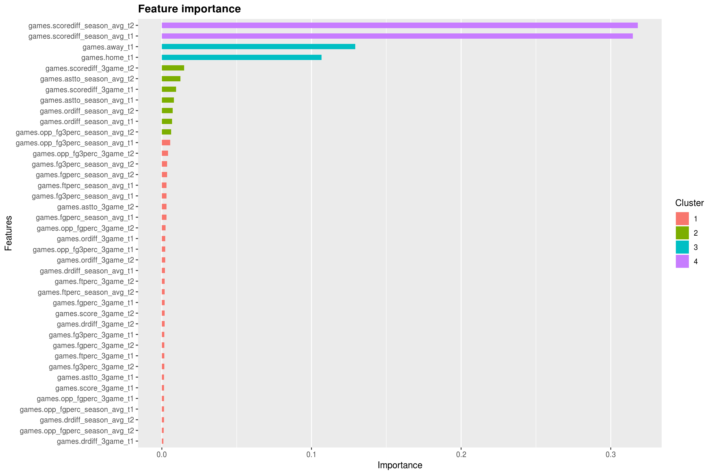
This plot gives us some insight as to what was important for the model to be able to accurately predict information. Even cooler, if you use the xgb.ggplot.importance function, it will cluster your variables based on importance. Not surprisingly, the average score differentials for the two teams was the most importing information for the model to have, and is the top cluster of variables. Next, was knowing if it was a home or an away game, also not surprising. It was interesting to see that assist to turnover ratio, offensive rebound differential, and 3 point shooting percentage emerged in a cluster above the other variables. Another cool feature is the tree plotting function. This one is a bit large, and I am only showing the first tree in the ensemble. You can use the trees parameter to show more.

xgb.plot.tree(
  feature_names = feature_names,
  model = xgb_reg,
  trees = 0
)

xgb.plot.multi.trees(
  model = xgb_reg,
  feature_names = feature_names
)

Conclusion

At the end of this series of posts, I don’t think I quite trust these models enough to start betting on college basketball games. This was a lot of fun to work on, and definitely challenging. My takeaways from this project, and my professional experience for that matter, is that the feature engineering side of data science is much more difficult and time consuming that the modeling side of things. As for using xgboost and keras for classification and regression tasks, I think I like xgboost a bit better, simply for the fact that I think it was a bit easier for me to use. From a performance perspective, we obviously saw very similar results.

To wrap up the work on this series of posts, I will be updating the shiny app that will have the clustering example baked in, as well as a tab to obtain predictions from each of the four models built in this series. As of right now, it will just be using the testing set that we used in this series, but if I come back to it in the future, I would like to have the ability to predict game outcomes on an ongoing basis. We’ll see if that ever happens…